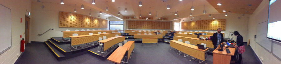
That’s right, we transcribed the talk we gave at the DH2015 in Sydney, on 2 July 2015, entitled “Digital Network Analysis of Dramatic Texts”. Please note that our grammar might appear a bit jetlagged here and there. ;) We were the last group to speak in a very interesting network-analysis centric session chaired by Glenn Roe. If you take a veeery close look (hehe) at this panorama pic, you will recognise us setting up the room together with the other speakers, Elisa Beshero-Bondar and Ryan Heuser (big hello there!):

Since we used reveal.js as presentation framework, we can easily reference individual slides so you can follow both our transcript and the slides simultaneously. (For further reference: Our original abstract can be found here.) But let’s now start with our presentation:

Slide 0/0: Title

Slide 1/0: TOC

1. Approach

Slide 2/0: Basic Ideas

The tradition of structural approaches in Literary Studies reaches back to (at least) the different flavours of European structuralism developed since the 1960s. Our project sets out to continue this tradition, but our new take on the issue is to apply an automated data analysis to identify and characterise structural features of literary texts, or, more precisely: of dramatic texts. The long-term objective of our project is to gather and provide structural data which can be used, for example, to describe different compositional types of plays. What we mean by compositional types, or, types of structural composition, is best illustrated by an example.

Slide 2/1: Different Styles of Structural Composition

Let’s have a look at these two network graphs generated during our data analysis. The graph on the left visualises the scenic interactions between characters in Goethe’s neo-classical play from 1787, “Iphigenie auf Tauris” (“Iphigenia in Tauris”), which is influenced by Aristotelian poetics. The graph on the right side visualises the interactions in a work also written by Goethe, the historical play “Götz von Berlichingen”, which, for his part, is strongly influenced by Shakespearean poetics. We cannot discuss this in detail here. But even at first glance you can clearly see the structural differences. The two works are composed in very different ways, exhibiting two very different types of structural or compositional style.

Slide 2/2: The Digital Spectator

In our project, we are looking into these different structural styles in the context of the history of dramatic texts. As mentioned before, we are stepping into the tradition of structuralistic approaches, and we combine these approaches with methods developed in the field of Social Network Analysis – as done by several scholars since the early 21st century, by de Nooy, Rydberg-Cox or Moretti, to name but a few. We are borrowing our specific definition of structure from Social Network Analysis, meaning: The structure of a dramatic text we are analysing originates from interactions between the characters in a play. To be more precise: A relation between two characters as we define it is given if both characters are performing a speech act in a given segment of a play, generally in a scene. So, if character A and character B are speaking in a scene, they are – following our definition – linked to each other.

This definition is inspired by works of Romanian mathematician Solomon Marcus. In his intriguing study “Mathematical Poetics” from 1973, Marcus suggests a concept which one might call “the digital spectator”. This is right up our alley, because with out digitally-driven method we are simulating this digital spectator who is not looking at a performance of the play on stage, but at an XML file. By means of our definition of interaction we are collecting our data; we are calculating network measures, generating graphs, running statistics and doing some other quantitative-analysis stuff.

Slide 2/3: 465 Network Graphs

And we are doing this, at the moment, with a corpus of 465 German-language plays – which you can see here. (By the way: You can download this fancy poster containing the network graphs of our whole corpus of 465 texts from figshare.) We are planning to include plays from other periods in our analysis, and we will, in the future, include plays written in other languages. But for the time being, our focus is on German plays from two centuries.

Slide 2/4: Workflow

Let’s now introduce our workflow and its three main steps: data mining, data editing and the display and analysis of our data.

2. Data Mining

Slide 3/0: Corpus

What makes our analysis quite difficult is that we are dealing with (excuse our French:) dirty data. If you happen to work with TEI documents like the ones from the Folger Shakespeare Library corpus, it’s pretty easy to do the kind of structural analysis we have in mind. But such a well-tagged TEI corpus is rare. Typically, we can consider ourselves lucky if we can obtain a digitised text of a focal text, and even luckier if it contains some basic markup. This applies, for example, to the bigger corpora containing German-language literature. For example, the quite large and freely available TextGrid Repository (comprising texts from around 1500 to the 1930s) features TEI markup converted automatically from a proprietary format. For that reason, we have to deal with quite a basic TEI markup and loads of different tagging errors. We had two options, basically: We could try to initiate a 6-figure project and manually improve the faulty tagging over several years; or, we could try to extract just the specific data we need and take it from there, improving just the bits essential for our approach. Lacking several hundreds of thousands of Euros, we chose the second way.

In order to build our corpus, we first had to extract all dramatic texts from the TextGrid Repository. This might sound relatively easy, but it’s not. We wrote a larger blog post on this subject, but to make it short: We ended up with 666 dramatic texts containing some basic TEI markup.

Slide 3/1: DLINA Corpus 15.07 (“Codename Sydney”)

Out of this corpus, we constructed our own subcorpus, its current version is entitled “DLINA Corpus 15.7 (Codename: Sydney)”. This corpus comprises 465 dramatic texts, so we discarded some 200 files. There are several reasons for excluding texts from our corpus. First, we wanted to limit our research to a specific time span, beginning with the modernisation of German drama at the outset of Enlightenment era, which means – following a well-established academic position – to start with the 1730s works of Johann Christoph Gottsched. We further ruled out foreign-language plays, translations, mere pantomime plays, and fragments. Plus, we sorted out a few texts with very defective TEI markup. All in all, our Sydney corpus comprises 465 dramatic texts in German language ranging from 1731 to 1929.

This was just our starting point. The next step was turned out to be another major task, the data editing.

3. Data Editing

Slide 4: Extracting Structural Data

As mentioned before, the TEI markup in the TextGrid Repository data was quite rudimentary – and often erroneous. So we had to find a way to edit and improve the data. Because we are just interested in a specific kind of structural data, we decided not to regularly edit the original XML files but to selectively extract those data we are interested in, and then just edit these specific data. This was the moment in which we invented what we call the “DLINA zwischenformat”, which roughly translates as DLINA intermediary format’, or simply ‘DLINA data file’. This intermediary format can be considered a structural abstraction of the fulltext TEI documents in our corpus. It is an XML file which is validated against a specific RNG schema. A zwischenformat file is created for each drama. It stores metadata, the actual structural data, and documentation (optional).

The structural data stored are the acts and scenes, the speakers occurring in the respective segments, and (optionally) some amounts, e.g., the number of speech acts, words, etc. for these characters. This DLINA data file not only makes improving the data quality easier but it also allows for a relatively quick way of gathering new data by basically just writing down the structure of a play and the speakers in the segments. You may have a look at our blog post that introduces the DLINA intermediary format. Or maybe you like to explore all the 465 DLINA files which we generated from our corpus and which are stored on GitHub.

Slide 4/1: Editing Process

However, just generating the DLINA data files was not enough. This is because the raw DLINA data files still retained some of the dirty data from the original XMLs – it was, in other words, full of bugs. So, manual intervention was often necessary to improve the data quality and correct errors in the source data.

In this editing process we had to face some errors that came about due to the automated conversion to TEI from the proprietary XML format; and we had to face some, so to say, intrinsic problems, i.e., characteristics typical for a play.

One recurrent problem of the first group were OCR errors in the <speaker> name. One of the phenomenons resulting from intrinsic characteristics of a play was that there were different ways of refer to a character. For example, a character’s full name might be given on the first appearance and only the first name on further appearances. In this case, we had to manually identify both names and attribute them to the one character they refer to.

There were a lot more problems we had to solve while editing the DLINA intermediary format. We established a larger set of editing rules, a complete documentation including examples can be found on our blog.

Slide 4/2: Outlook

We will further improve our editing process. At this time, for example, we are developing a GUI for some of the more simple editing procedures. This GUI will also include some gamification elements, so maybe we will have some crowd-editing-option in the future.

4. Display and Analysis

Slide 5/0: Four Types of Visualisation

After editing and cleaning our 465 data files, we did two things: We started to publish our data and commented on it in larger blog posts, and we ran some statistics, also with detailed comments. As we stressed before and can’t stress enough, this project is still very much a work in progress, but we can and we will show you some promising first results. As mentioned before, all our data is stored on our GitHub, and therefore very transparent. On top of that, we built a small network-data publishing machine to provide easy access to our data. We created a homepage for every of the 465 plays. There is a list of all these plays if you click on this link. On each of the homepages you’ll find 4 links leading to further information on the particular play.

Slide 5/1: Example: G. E. Lessing’s “Emilia Galotti” (1772)

One of the pages shows the network graph, with edges between all the people speaking in the same segment. There is a static graph and one with sticky nodes. Another page shows a matrix of encounters. And there is a page where you can have a look at our intermediary source file. That’s our data in plain daylight! Eventually, there is one page that contains a bar chart with word counts for each character of the play. You can also interactively sort them.

Slide 5/2: Skit (The Biggest Chatterboxes in German Literature)

Which brings me to a little skit, a little interlude. With the kind of data we gathered, it was easy for us to make a list of the biggest chatterboxes in German literature, of course, only based on our middle-sized corpus. And for all of you who didn’t do their German Literature 101: It doesn’t matter, I’m sure you will at least know Faust and his counterpart Mephistopheles, from Goethe’s play “Faust, part 1”. And both of them are very talkative, earning places 3 and 4 of this top-10 of the biggest chatterboxes in German literature. Again, there’s a blog post on the subject, but of course, this one is a bit “tongue-in-cheek” and not part of our actual research.

Let’s rather have a look at some more meaningful facts. We actually started out to process our data by means of Social Network Analysis. Again, our measures are currently very basic, for example, we’re computing the size of our drama networks, their density, their average degree and so on. For now, let us acquaint you with just two charts we’re currently discussing in the group and with other colleagues.

Slide 5/3: Network Size (Median) by Decade (1730–1930)

Here you can see the evolution of network sizes between 1730 and 1930. On the x-axis you can see the 20 decades. The y-axis features the median values of the number of characters of all the plays of a decade.

Let’s now try some cautious-cautious interpretation of this diagram. Something is happening there, that’s for sure, but what exactly? Well, some of the ups and downs we did expect. Like for example: The increase of this value in the second half of the 18th century might be associated with the beginning reception of Shakespeare in Germany, which lead, among other things, to the rise of the Historical Play in German literature. Or, another quick glimpse, the dropping values at the end of the 19th century might be associated with the rise of the Naturalistic Drama, which – to make a long story short – returned to the ideas of something like a Aristotelian poetics.

We published many more charts on our website, we also started to discuss them there, and this process will continue, of course. If you like, please have a look – and join the discussion. For now, we just show you one last chart, one that introduces another idea we will address with our statistical approaches. I’m talking about concepts of genre, or rather: subgenre.

Slide 5/4: Network Density (Mean) by Genre and Century

While editing our intermediary files we also included basic genre data, with the main focus on the usual suspects, major genres like tragedy, comedy, and opera libretti. With this kind of genre data we could now build subcorpora to have a look at genres and their specific network measures.

And we immediately noticed some interesting things. What we can see here is a multiple-line chart featuring the arithmetic means of density values by genre and century. Just looking at this single value over time, we can conclude that comedies and libretti implement a very similar structural composition over the centuries, while character networks of tragedies (the lowermost line in our diagram) show a much lower density. What is more, the values shown are pretty consistent over the centuries. This might be a first indication that we could actually cluster genres of dramatic texts by just looking at a few basic measures.

But as stated before, today we’re only talking about very basic data. Actually, we calculated a lot more network data and started to look into them. But we should not run to conclusions too fast. It is still a long way to integrate our network analysis of dramatic texts into a holistic study of literary evolution. We will be pushing out more data on our blog in the next few months. For example, we’re putting the finishing touches on an article on Network Values by Genre, should be ready in two weeks or three.

5. Further Research

Slide 6/0: Yada Yada

Wrapping things up, here is a slide with some notes on further research ideas. We need more statistical data, and we need to interpret them thoroughly. In addition, we will enlarge our German-language corpus. We will also look into existing foreign-language corpora which also opens up the field of comparative studies. I’m especially thinking of Paul Fièvre’s excellent corpus comprising more than 750 French plays, but we will also be looking into a collection of American drama and we’re also happy to cooperate with other scholars on the subject. But our first and foremost task will be to find ways to contribute to traditional Literary Studies, to evaluate existing hypotheses reached by close-reading approaches, by traditional means, so to speak. Plus, we will try to reach an own set of interpretations and hold them against established hypotheses in the field of Literary Studies. That is and should be our long-term plan at least.

6. Bibliography

Slide 7/0: Literary Theory, Social Network Analysis

Slide 7/1: Literary Studies & SNA

Slide 7/2: Literary Studies & SNA (Cont’d)

That was it. Thanks a lot for all the feedback we got, for the nice talks after the session and throughout the whole conference. Also if we aren’t even halfway there, it is nice to see how the network analysis of literary texts progresses. It’s definitely something to look out for at upcoming DH conferences.